Nodal Analyses Reference
Introduction
In the following discussion we assume that  is the vector of
nodal variables. We denote matrices and frequency-domain quantities
with uppercase letters.
is the vector of
nodal variables. We denote matrices and frequency-domain quantities
with uppercase letters.
This section documents the formulation used for nodal-based analyses. For all analyses there are four types of devices to consider:
Linear VCCS/QS
Contribute theand
matrices, respectively. Elements provide the following attributes to build these matrices: linearVCCS and linearVCQS.
Nonlinear VCCS/QS
Contribute
and
vector functions. Here
is a vector with controlling port voltages and
is a vector with time-delayed control voltages. For the
nonlinear device, vector
and its Jacobian are returned by eval_and_deriv(). The Jacobian is returned in a single matrix with the following format:
In nodal analyses, controlling port voltages (
where
is an incidence matrix. All nonzero entries in
are either equal to 1 or -1 and there are at most two nonzero entries per row. This matrix is implicitly stored in the simulator with the control port definitions in each element. Samples of time-delayed control voltages can be calculated in a similar way using a
Vector functions
and
, which have the same properties as the transpose of
![\left[ \begin{array}{cc} di_j/dv & di_j/dv_T \\
dq_j/dv & dq_j/dv_T
\end{array} \right]](_images/math/b59f0fc8d2b17ef480277fdcfdfcc6d3336bf6e8.png)

Frequency-defined devices
Contribute the complex, frequency-dependentmatrix. The corresponding impulse-response matrix is denoted
. The following methods are used to build this matrix: get_Y_matrix() for
and get_G_matrix() for
. More details will be provided when time-domain support for this kind of device is implemented.
Sources
Contribute a source vector. There are 3 types of source: DC (), time-domain (
) and frequency-domain (
). The following element methods are used: get_DCsource(), get_TDsource(), get_FDsource() and get_AC().
OP/DC Equations
For DC analysis, time-delayed control voltages are calculated as
regular control voltages; and are ignored
and only the DC component of sources () and the DC
conductance matrix of frequency-defined elements ( ) are
considered.
) are
considered.
The analysis solves the following nonlinear equation iteratively using Newton’s method:

Let 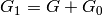 . The iteration is defined by linearizing
 as follows:

where the  superscript indicates the iteration number and
The  vector is assumed to be known for each iteration and
 is the unknown to solve for. The initial guess
(
is the unknown to solve for. The initial guess
( ) is set to the values suggested by the nonlinear devices,
if any, or otherwise to zero. The previous equation can be re-arranged
as as the following system of linear equations:
) is set to the values suggested by the nonlinear devices,
if any, or otherwise to zero. The previous equation can be re-arranged
as as the following system of linear equations:

with 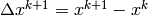 . This equation can be
seen as the nodal equation of a linearized circuit obtained by
substituting all devices by transconductances in parallel with current
sources that are dependent of the current approximation for the nodal
voltages ().
. This equation can be
seen as the nodal equation of a linearized circuit obtained by
substituting all devices by transconductances in parallel with current
sources that are dependent of the current approximation for the nodal
voltages ().
The condition to stop Newton iterations is:

for each nodal variable ( ). In addition, if errfunc is
set to True, nodal equations are also checked:
). In addition, if errfunc is
set to True, nodal equations are also checked:

and iterations stop when both conditions are satisfied. Normally the first condition is enough to obtain an acceptable solution and that is why by default the second check is not enabled to save the CPU time required to re-evaluate the nodal equations.
AC Formulation
Here  is the nodal vector in frequency domain. A DC
operating point analysis is performed first to obtain the incremental
conductances and capacitances given by
is the nodal vector in frequency domain. A DC
operating point analysis is performed first to obtain the incremental
conductances and capacitances given by  and
and
 , respectively. The analysis solves for for
all requested frequencies using the following equation:
, respectively. The analysis solves for for
all requested frequencies using the following equation:
![\left[ (G + J_i + j 2 \pi f (C + J_q)
+ Y(f) \right] \, X(f) = S(f)](_images/math/1ef2924cf1fb0caa5a8f622df0192eb11e13750c.png)
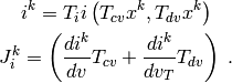
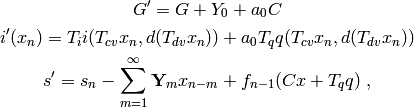
The  and
and  Jacobian matrices are calculated as
follows:
Jacobian matrices are calculated as
follows:
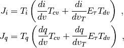
where  is a diagonal matrix that includes the effect
of time delays in each control port:
is a diagonal matrix that includes the effect
of time delays in each control port:
![E_{\tau} = \mbox{diag}\left( [\exp(-j \omega \tau_1),
\exp(-j \omega \tau_2), \dots , \exp(-j \omega \tau_m)]
\right)](_images/math/becad078042b733385aa0ceba06d6476a4cfb4b7.png)
Transient Analysis Equations
Transient analysis solves the following nonlinear
algebraic-integral-differential equation given an initial condition,
 :
:

where dotted quantities indicate derivative with respect to time and
 is a vector function that applies a (possibly different)
time delay to each control voltage. The delay function ()
is implemented by storing all time-delayed control port voltages and
using an interpolation function to find the voltage at the desired
time in the past.
is a vector function that applies a (possibly different)
time delay to each control voltage. The delay function ()
is implemented by storing all time-delayed control port voltages and
using an interpolation function to find the voltage at the desired
time in the past.
The initial condition ( ) is usually obtained by
calculating the operating point of the circuit using the OP analysis.
) is usually obtained by
calculating the operating point of the circuit using the OP analysis.
An integration method such as Backward Euler (BE) or trapezoidal rule
is applied to transform the differential equation into a difference
equation by discretizing time and approximating derivatives with
respect to time. Here we assume the time step ( ) is constant.
For example, using the BE rule:
) is constant.
For example, using the BE rule:
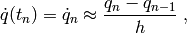
here, the subscript  denotes the time sample number. For
implicit methods in general,
denotes the time sample number. For
implicit methods in general,
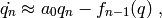
with  being a function that depends on the previous
samples of
being a function that depends on the previous
samples of  :
:

The 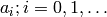 coefficients depend on the time step size
and the integration method. Substituting dotted variables and
discretizing the convolution operation the resulting circuit equation
is the following:
coefficients depend on the time step size
and the integration method. Substituting dotted variables and
discretizing the convolution operation the resulting circuit equation
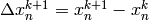
is the following:
with
where  and
and  . Note that
 is a known vector at the
  time step. This is
the equation of a DC circuit with a conductance matrix equal to
time step. This is
the equation of a DC circuit with a conductance matrix equal to
 , a set of nonlinear currents given by the
  function and a source vector given by . The unknown
(
function and a source vector given by . The unknown
( ) is iteratively solved using Newton’s Method (similarly
as in OP/DC analysis). Iterations are defined by linearizing
) is iteratively solved using Newton’s Method (similarly
as in OP/DC analysis). Iterations are defined by linearizing
 as follows:

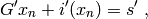
where the subscript denotes the Newton iteration number,
 and
and 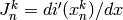 . This equation is re-arranged as follows:

as the right-hand side of this equation is known at the  iteration,
  can be found by solving a linear system
of equations.
can be found by solving a linear system
of equations.
The criterion to stop iterations is the same as in the DC analysis.