Simulation Examples

The following examples give an idea of the current simulator capabilities shortly after version 0.3.dev. Some of these results may change as errors are discovered and fixed or new capabilities are added.

DC Sweep of CMOS Inverter

The netlist is the following:

# CMOS inverter DC Sweep

.analysis dc device=vdc:vin param=vdc start=0 stop=3V

vdc:vdd 1 gnd vdc=3V
vdc:vin in gnd vdc=1

x1 in out 1 gnd inverter

.subckt inverter in out vdd vss
mosekv:m1 out in vdd vdd type = p
mosekv:m2 out in vss vss type = n
.ends

.plot dc out

.end

Running this netlist produces the following output:

cechrist@moon:~/wd/cardoon/examples$ cardoon inverter.net

Cardoon Circuit Simulator 0.5 release 0.5.0.dev
******************************************************
                 DC sweep analysis
******************************************************

 # CMOS inverter DC Sweep

System dimension: 5
Sweep:  Device: vdc:vin  Parameter: vdc
Average iterations: 3
Average residual: 5.33145579173e-06

dc analysis time: 0.48 s

Press [Enter] to exit ...

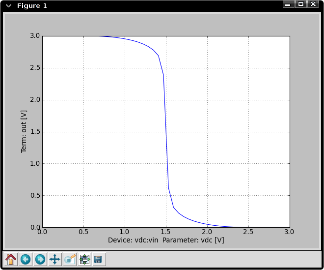
The output plot of the inverter’s output voltage is shown below.

BJT Colpitts Oscillator Transient Analysis

Netlist:

### BJT Colpitts Oscillator ###

# Voltage supply: use a pulse to start oscillator
vpulse:vs 1 0 v1=3 v2=11 tr=10ns

res:rc 1 2 r=2.4e3
cap:c1 2 0 c=2e-12
ind:l1 2 5 l=1e-6
cap:c2 5 0 c=2e-12
res:re 4 0 r=1.3e3
cap:ce 4 0 c=100e-12
bjt:q1 2 3 4 model=t122
res:r1 1 3 r=8e3
res:r2 3 0 r=2e3
cap:cc 5 3 c=400e-12

.model t122 bjt (type=npn isat=0.480e-15 nf=1.008 \
bf=99.655 vaf=90.000 ikf=0.190 \
ise=7.490e-15 ne=1.762 nr=1.010 br=38.400 var=7.000 ikr=93.200e-3 \
isc=0.200e-15 nc=1.042 rb=1.500 irb=0.100e-3 rbm=1.200 cje=1.325e-12 \
vje=0.700 mje=0.220 fc=0.890 cjc=1.050e-12 vjc=0.610 mjc=0.240 xcjc=0.400 \
tf=56.940e-12 tr=1.000e-9 xtf=68.398 vtf=0.600 itf=0.700 xtb=1.600 \
eg=1.110 xti=3.000 re=0.500 rc=2.680)

.analysis tran tstop=50ns tstep=20ps im=trap

.plot tran 2 3

.end

Running this netlist produces:

cechrist@phobos:~/src/cardoon/examples$ cardoon oscillator.net
******************************************************
                 Transient analysis
******************************************************

 ### BJT Colpitts Oscillator ###

System dimension: 11


Average iterations: 3
Average residual: 2.55259547323e-09

The output plot of the collector (blue) and base (green) voltages is shown below.

Electro-Thermal BJT Test

The following netlist illustrates the electro-thermal version of the BJT model:

# Test of an electrothermal BJT

.analysis dc device=vdc:vb param=vdc start=0 stop=12 shell=1

.model mynpn svbjt_t (bf=200 vaf=100 ikf=10e-3 rb=1k)

vdc:vce 10 gnd vdc=12
res:rc 10 1 r=1k
vdc:vb 3 0 vdc=10
res:rb 3 2 r=96k

svbjt_t:q1 1 2 0 0 t1 gnd model=mynpn

res:rth t1 0 r=100.

.plot dc t1
.plot dc 1 2

.end

Note that shell=1 in the analysis line. This indicates the simulator to run an interactive shell after completing the analysis. Running this netlist and entering some commands in the simulator shell produces:

cechrist@moon:~/wd/cardoon/examples$ cardoon npn_thermal.net

Cardoon Circuit Simulator 0.4 release 0.4.1.dev
******************************************************
                 DC sweep analysis
******************************************************

 # Test of an electrothermal BJT

System dimension: 11
Sweep:  Device: vdc:vb  Parameter: vdc
Average iterations: 5
Average residual: 0.0114478106429

Dropping into IPython, type CTR-D to exit
Available commands:
    sweepvar: vector with swept parameter
    getvec(<terminal>) to retrieve results
    plt.* to access pyplot commands (plt.plot(x,y), plt.show(), etc.)

In <1>: ic = (getvec('10') - getvec('1')) / 1000.
In <2>: plt.plot(sweepvar,ic)
Out<2>: [<matplotlib.lines.Line2D object at 0xa7c3a4c>]
In <3>:

The shell commands above produce a plot of the collector current. All matplotlib and ipython commands are available in the shell. Note that you must first close the initial plots to get the shell prompt.

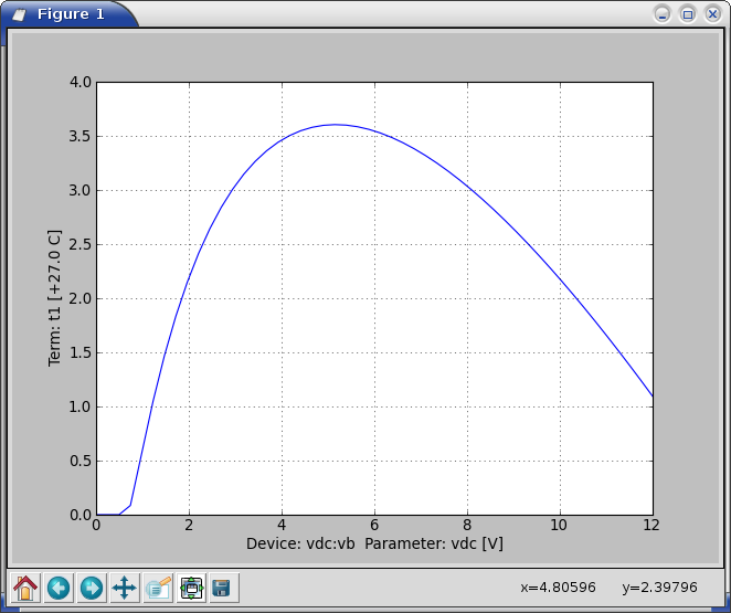
The base voltage is swept. As the collector current increases, at first the power dissipation in the BJT also increases but eventually the reduction in causes a reduction in power dissipation as the transistor gets closer to saturation. This effect can be observed in the temperature plot shown below. Temperature is given as the increment to ambient temperature given in the .options line (the default value is used here).

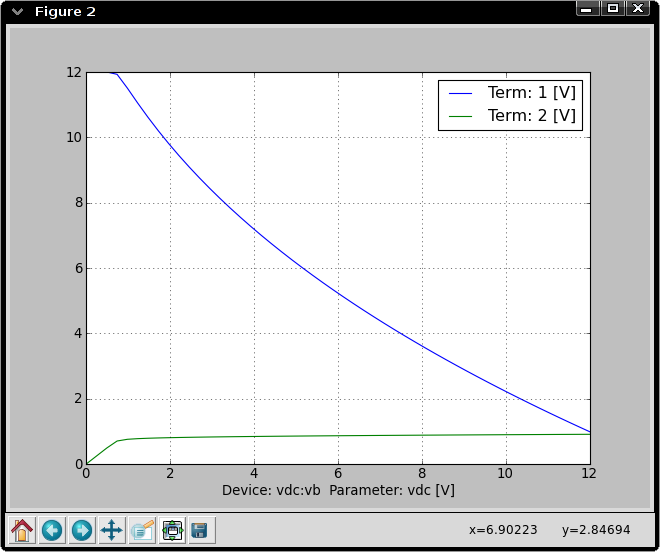
The collector and base voltages are shown below:

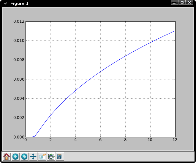
Collector current plot:

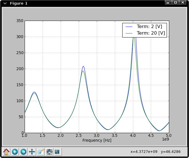
Transmission Line Model AC test

The following netlist compares two transmission line models: one based on RLGC sections and the other based on the scattering parameters. Two identical circuits are used:

# Simple netlist with transmission line (test of nsect parameter)

isin:i1 gnd 4 idc=2m acmag=1.
res:r1 4 2 r=100
tlinpy4:tline1 2 gnd 3 gnd nsect=50 tand=1e-3 z0mag=50
res:r2 3 gnd r=100
svdiode:d1 3 gnd cj0=1e-12

isin:i10 gnd 40 idc=2m acmag=1.
res:r10 40 20 r=100
tlinps4:tline10 20 gnd 30 gnd tand=1e-3 z0mag=50
res:r20 30 gnd r=100
svdiode:d10 30 gnd cj0=1e-12

.analysis ac start=1GHz stop=5GHz num=200 log=False shell=0

.plot ac_mag 2 20
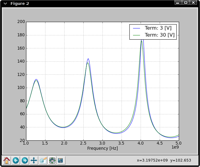
.plot ac_mag 3 30

.end

Run netlist:

cechrist@phobos:~/src/cardoon/examples$ cardoon tlinpy.net
******************************************************
                 AC sweep analysis
******************************************************

 # Simple netlist with transmission line (test of nsect parameter)

The following are the plots comparing the input and output voltages of the two circuits:

Memductor Hysteresis Loop

This circuit is composed of an ideal sinusoidal voltage source connected to a memductor (or flux-controlled memristor):

# Simple netlist to test memductor

vsin:vin 1 0  mag=4.5 freq=10Hz phase=-90
memd:w1 1 0 w = '3 * phi*phi + .1 * abs(phi) + 3e-3'

.analysis tran tstep=1ms tstop=95ms shell=1

.plot tran 1
.plot tran vsin:vin:i

.end

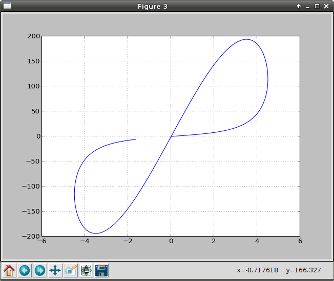
# In the shell, run the following commands to plot hysteresis loop:
import matplotlib.pyplot as plt
plt.figure()
plt.plot(getvec('1'), -getvec('vsin:vin:i'))

Note that any lines after .end are ignored by the simulator. Running this netlist produces the plots of the voltage and current in the memductor:

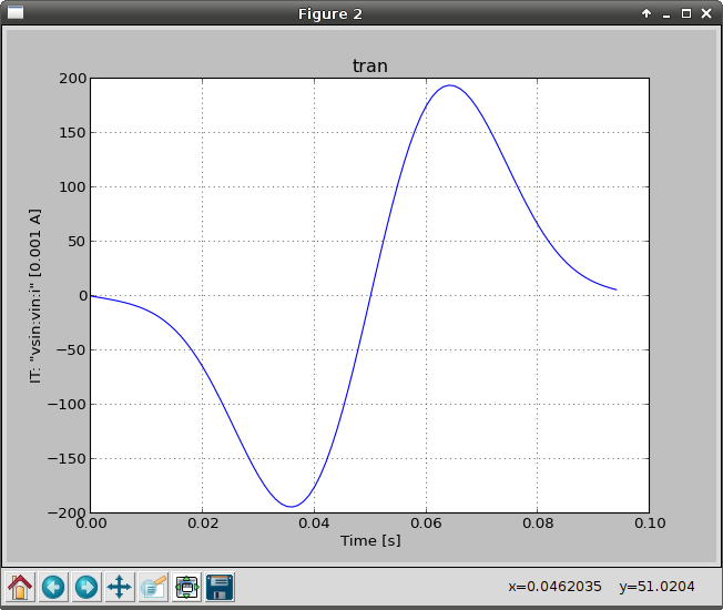
Executing the commands listed at the end of the netlist in the shell produces the hysteresis loop (type ‘g’ in the graph window to turn on the grid). The stop time in the transient analysis is set to be less than one period in order to visualize the direction of the loop:

Examples Directory

The examples directory contains ready-to-use netlist examples. They all should work with no errors. To run netlists, execute the following command:

cardoon/examples$ ../cardoon.py <netlist file>

Brief description of each file:

1. inverter.net: Basic CMOS inverter from documentation (DC sweep)
2. npn_thermal.net: Electro-thermal BJT test from documentation (DC sweep). Simulation drops to an ipython shell at the end. Results can be explored with more detail in this mode. Type quit() to exit this shell.
3. oscillator.net: Colpitts oscillator from documentation (transient)
4. ring_osc_ahkab.net: CMOS ring oscillator similar to the example provided with the ahkab <http://code.google.com/p/ahkab/> simulator.
5. summing_lm741.net: transistor-level LM741-based summing amplifier (transient)
6. thermal_rf_amp_AC.net: RF amplifier with transmission lines (AC sweep)
7. soliton.net: Nonlinear transmission line transient simulation. This simulation takes approximately 5 minutes to complete.
8. lma411.net: X-Band MMIC amplifier.
9. memductor.net: illustrates the behaviour of a memductor and how to use simulation results in an interactive shell